Getting Started
With Tools
Marvin Galaxy Tools are the four main classes (Cube, RSS, Maps, and ModelCube) associated with the analogous DRP and DAP data products, the Astropy quantities representing multidimensional data, and a variety of utilities and mixins that provide additional functionality. Sub-region galaxy tools (Spaxel and binning information) are explained in their own section. The four main Tools classes inherit from MarvinToolsClass and thus much of their functionality and logic is shared. In this section we will prominently use the Cube but most of what we explain here also applies to the remaining Tools.
All the Tools classes can be accessed from the marvin.tools module. Let’s load a DRP Cube
>>> import marvin
>>> my_cube = marvin.tools.Cube('8485-1901')
>>> my_cube
<Marvin Cube (plateifu='8485-1901', mode='local', data_origin='file')>
Depending on whether you have the file on disk or not, the access mode will be 'local' or 'remote'. Regardless of that, the way we interact with the object will be the same. All tools provide quick access to some basic metadata
>>> print(my_cube.filename, my_cube.plateifu, my_cube.mangaid, my_cube.release)
/Users/albireo/Documents/MaNGA/mangawork/manga/spectro/redux/v2_3_1/8485/stack/manga-8485-1901-LOGCUBE.fits.gz 8485-1901 1-209232 DR15

>>> print(my_cube.ra, my_cube.dec)
232.544703894 48.6902009334
Similarly we can access the header of the file and the WCS object
>>> my_cube.header
XTENSION= 'IMAGE   '           / IMAGE extension
BITPIX  =                  -32 / Number of bits per data pixel
NAXIS   =                    3 / Number of data axes
NAXIS1  =                   74 /
NAXIS2  =                   74 /

>>> my_cube.wcs
WCS Keywords

Number of WCS axes: 3
CTYPE : 'RA---TAN'  'DEC--TAN'  'WAVE-LOG'
CRVAL : 232.5447  48.690201  3.62159598486e-07
CRPIX : 18.0  18.0  1.0
CD1_1 CD1_2 CD1_3  : -0.000138889  0.0  0.0
CD2_1 CD2_2 CD2_3  : 0.0  0.000138889  0.0
CD3_1 CD3_2 CD3_3  : 0.0  0.0  8.33903304339e-11
NAXIS : 34  34  4563
What is more, we can access the datamodel of the cube file, which show us what extensions are available, how they are named in Marvin, and what they contain
>>> datamodel = my_cube.datamodel
>>> datamodel
<DRPCubeDataModel release='DR15', n_datacubes=3, n_spectra=2>

>>> datamodel.datacubes
[<DataCube 'flux', release='DR15', unit='1e-17 erg / (Angstrom cm2 s spaxel)'>,
 <DataCube 'dispersion', release='DR15', unit='Angstrom'>,
 <DataCube 'dispersion_prepixel', release='DR15', unit='Angstrom'>]

>>> datamodel.spectra
[<Spectrum 'spectral_resolution', release='DR15', unit='Angstrom'>,
 <Spectrum 'spectral_resolution_prepixel', release='DR15', unit='Angstrom'>]
This tells us that this cube has two associated 3D datacubes, 'flux', 'dispersion', and 'dispersion_prepixel', and two associated spectra, 'spectral_resolution' and 'spectral_resolution_prepixel', as well as their associated units. We can get a desciption of what each of them
>>> datamodel.datacubes.flux.description
'flux'
>>> datamodel.datacubes.flux.description
'3D rectified cube'
In my_cube, we can use the name of each of these datacubes and spectra to access the associated data quantity. Let’s get the cube flux
>>> flux = my_cube.flux
>>> flux
<DataCube [[[0., 0., 0., ..., 0., 0., 0.],
            [0., 0., 0., ..., 0., 0., 0.],
            [0., 0., 0., ..., 0., 0., 0.],
            ...,
            [0., 0., 0., ..., 0., 0., 0.],
            [0., 0., 0., ..., 0., 0., 0.],
            [0., 0., 0., ..., 0., 0., 0.]]] 1e-17 erg / (Angstrom cm2 s spaxel)>
The flux is represented as a 3D array with units. We can also access the inverse variance and the mask using flux.ivar and flux.mask, respectively. We can slice this datacube to get another datacube
>>> flux[:, 50:60, 50:60]
<DataCube [[[ 0.23239002,  0.21799691,  0.1915081 , ...,  0.06516988,
          0.03220467,  0.02613733],
        [ 0.2511523 ,  0.25672358,  0.24318442, ...,  0.07530793,
          0.0505379 ,  0.05970671],
        [ 0.24604724,  0.23915106,  0.24392547, ...,  0.1116344 ,
          0.08573902,  0.10379973],
        ...,
        [ 0.        ,  0.        ,  0.        , ...,  0.        ,
          0.        ,  0.        ],
        [ 0.        ,  0.        ,  0.        , ...,  0.        ,
          0.        ,  0.        ],
        [ 0.        ,  0.        ,  0.        , ...,  0.        ,
          0.        ,  0.        ]]] 1e-17 erg / (Angstrom cm2 s spaxel)>
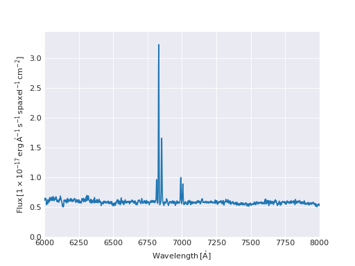
Or get a single spectrum and plot it:
>>> spectrum = flux[:, 50, 55]
>>> spectrum
<Spectrum [0.1060614 , 0.07801704, 0.02460545, ..., 0.16328742, 0.13772544,
       0.        ] 1e-17 erg / (Angstrom cm2 s spaxel)>

>>> spectrum.plot(show_std=True)
(Source code, png, hires.png, pdf)
We will talk more about quantities in the Working with Astropy Quantities section, and about more advance plotting in marvin-plotting.
From a DRP cube we can get the associated DAP Maps object for a certain bintype
>>> hyb_maps = my_cube.getMaps(bintype='HYB10')
<Marvin Maps (plateifu='8485-1901', mode='local', data_origin='file', bintype='HYB10', template='GAU-MILESHC')>
A Maps behaves very similarly to a Cube and everything we have discussed above will still work. Instead of datacubes and spectra, a Maps object contains a set of 2D quantities called Map, each one of them representing a different property measured by the DAP. One can get a full list of all the properties available using the datamodel
>>> hyb_maps.datamodel
[<Property 'spx_skycoo', channel='on_sky_x', release='2.1.3', unit='arcsec'>,
 <Property 'spx_skycoo', channel='on_sky_y', release='2.1.3', unit='arcsec'>,
 <Property 'spx_ellcoo', channel='elliptical_radius', release='2.1.3', unit='arcsec'>,
 <Property 'spx_ellcoo', channel='r_re', release='2.1.3', unit=''>,
 <Property 'spx_ellcoo', channel='elliptical_azimuth', release='2.1.3', unit='deg'>,
 <Property 'spx_mflux', channel='None', release='2.1.3', unit='1e-17 erg / (cm2 s spaxel)'>,
 <Property 'spx_snr', channel='None', release='2.1.3', unit=''>,
 <Property 'binid', channel='binned_spectra', release='2.1.3', unit=''>,
 ...
]
Note that some properties such as 'spx_skycoo' have multiple channels (in this case the on-sky x and y coordinates). We can get more information about a property
>>> hyb_maps.datamodel.spx_skycoo_on_sky_x.description
'Offsets of each spaxel from the galaxy center.'
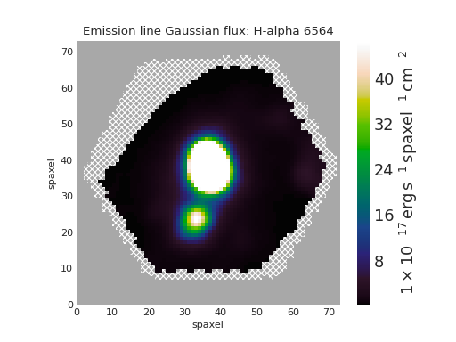
See the datamodel section for more information on how to use this feature. We can retrieve the map associated to a specific property directly from the Maps instance. For example, let’s get the H \(\alpha\) emission line flux (fitted by a Gaussian) from a different Maps file
>>> my_cube = marvin.tools.Maps('7443-12703')
>>> ha = my_cube.emline_gflux_ha_6564
>>> ha
<Marvin Map (property='emline_gflux_ha_6564')>
[[0. 0. 0. ... 0. 0. 0.]
 [0. 0. 0. ... 0. 0. 0.]
 [0. 0. 0. ... 0. 0. 0.]
 ...
 [0. 0. 0. ... 0. 0. 0.]
 [0. 0. 0. ... 0. 0. 0.]
 [0. 0. 0. ... 0. 0. 0.]] 1e-17 erg / (cm2 s spaxel)
Hint
In IPython, you can use tab-completion to autocomplete the name of the property. If you press tab after writing hyb_maps.emline_ you will get a list of all the emission line properties available.
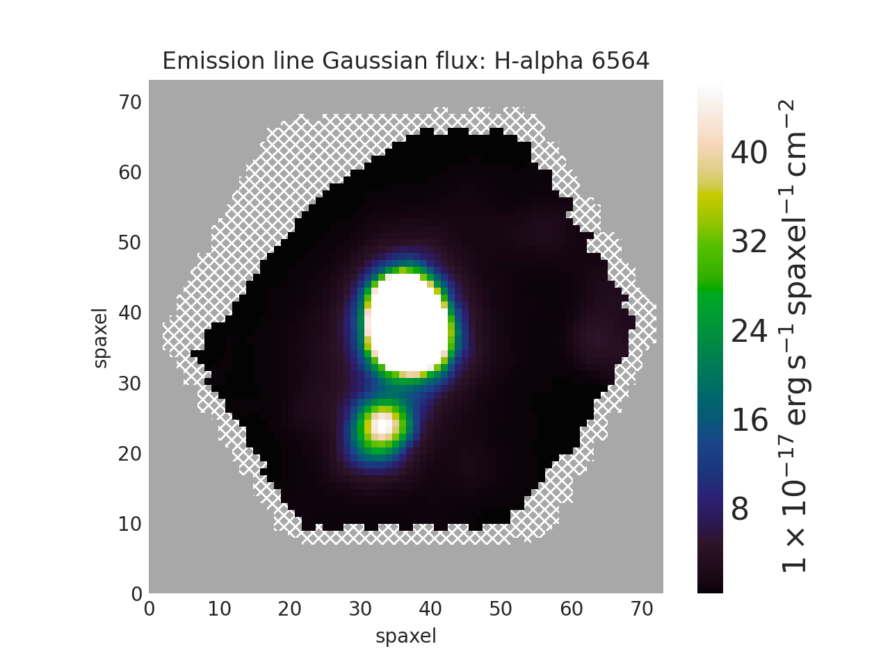
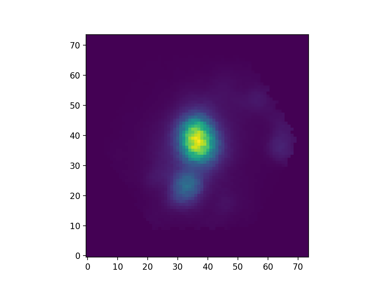
Map quantities are similar to DataCube but wrap a 2D array. We can plot the Map as
>>> fig, ax = ha.plot()
(Source code, png, hires.png, pdf)

Note that the plot method returns the matplotlib Figure and Axes for the plot. We can use those to modify or save the plot. Marvin plotting routines try to select the best parameters, colour maps, and dynamic ranges. You can modify those by passing extra arguments to plot. You can learn more in the Map plotting section. We will talk about the Map class in detail in Working with Astropy Quantities and in Map.
Let’s take a step back and go back to hyb_maps, our Maps instance. We can access the targeting bits for that galaxy (for an introduction to maskbits check this page)
>>> hyb_maps.target_flags
[<Maskbit 'MANGA_TARGET1' ['PRIMARY_PLUS_COM', 'COLOR_ENHANCED_COM', 'PRIMARY_v1_1_0', 'COLOR_ENHANCED_COM2', 'PRIMARY_v1_2_0']>,
 <Maskbit 'MANGA_TARGET2' []>,
 <Maskbit 'MANGA_TARGET3' []>]
Note that in this case the galaxy belongs to the primary sample from the final target selection (PRIMARY_v1_2_0) as well as to the primary and colour enhanced samples from several commissioning target selections. The galaxy does not have any ancillary bit (manga_target3).
Similarly, we can access quality flags, which indicate us if there is something we need to know about the data
>>> hyb_maps.quality_flag
<Maskbit 'MANGA_DAPQUAL' []>
In this case the MANGA_DAPQUAL maskbit does not have any bit activated, which means the data is safe to use. See the Maskbits section for more information.
For each target we can also access additional catalogue data: the associated parameters from the NASA Sloan Atlas, and the DAPall file
>>> my_cube.nsa
{'iauname': 'J151806.10+424438.0',
 'field': 213,
 'run': 3918,
 'camcol': 3,
 'version': 'v1_0_1',
 'nsaid': 684509,
 'nsaid_v1b': 230855,
 'z': 0.0402719,
 'zdist': 0.0406307,
 ... }

>>> my_maps.dapall
{'plate': 7443,
 'ifudesign': 12703,
 'plateifu': '7443-12703',
 'mangaid': '12-193481',
 'drpallindx': 1465,
 'mode': 'CUBE',
 'daptype': 'HYB10-GAU-MILESHC',
 ... }
The NSA and DAPall catalogues are implemented as mixins via NSAMixIn and DAPAllMixIn, respectively.
While Marvin allows you to access data remotely, frequently you will find that you want to download the file associated to an object so that you can access it more quickly in the future. We can do that using the MarvinToolsClass.download method. Let’s try to load a cube that we know we do not have in out hard drive
>>> remote_cube = marvin.tools.Cube('8485-1902')
>>> remote_cube
<Marvin Cube (plateifu='8485-1902', mode='remote', data_origin='api')>

>>> remote_cube.download()
SDSS_ACCESS> syncing... please wait
SDSS_ACCESS> Done!
Now we can try loading it again
>>> new_cube = marvin.tools.Cube('8485-1902')
>>> new_cube
<Marvin Cube (plateifu='8485-1902', mode='local', data_origin='file')>
>>> new_cube.filename
'/Users/albireo/Documents/MaNGA/mangawork/manga/spectro/redux/v2_3_1/8485/stack/manga-8485-1902-LOGCUBE.fits.gz'
The cube has now been loaded from the file we just downloaded! You can find the file in its corresponding location in your local SAS.
Finally, we can extract one or more Spaxel object from a Galaxy Tool. We can either use the standard array slicing notation (0-indexed, origin of coordinates in the lower left corner of the array)
>>> spaxel = new_cube[15, 10]
>>> spaxel
<Marvin Spaxel (plateifu=8485-1902, x=10, y=15; x_cen=-6, y_cen=-1, loaded=cube/maps)>
or we can use getSpaxel, which accepts multiple arguments (refer to the method’s documentation). Note that by default, (x, y) coordinates passed to getSpaxel are measured from the centre of the array
>>> central_spaxel = new_cube.getSpaxel(x=0, y=0)
>>> central_spaxel
<Marvin Spaxel (plateifu=8485-1902, x=16, y=16; x_cen=0, y_cen=0, loaded=cube/maps)>
Spaxel and Bin will be treated in detail in the marvin–subregion-tools section.
Working with Astropy Quantities
Marvin presents scientific data in the form of Astropy Quantities. A Quantity is essentially a number with an associated physical unit. In Marvin we expand on that concept and extend the Quantities with a mask, an inverse variance (why do we use ivar in MaNGA?) and, when relevant, the associated wavelength. Marvin Quantities also provide useful methods to, for instance, calculate the SNR or plot the value. Marvin provides Quantities for 1D (Spectrum, AnalysisProperty), 2D (Map), and 3D data (DataCube).
All Quantities behave similarly. Let’s start by getting a datacube (3D Quantity) from a Cube object
>>> my_cube = marvin.tools.Cube('7443-12701')
>>> flux = my_cube.flux
>>> flux
<DataCube [[[0., 0., 0., ..., 0., 0., 0.],
            [0., 0., 0., ..., 0., 0., 0.],
            [0., 0., 0., ..., 0., 0., 0.],
            ...,
            [0., 0., 0., ..., 0., 0., 0.],
            [0., 0., 0., ..., 0., 0., 0.],
            [0., 0., 0., ..., 0., 0., 0.]],

            ...,

           [[0., 0., 0., ..., 0., 0., 0.],
            [0., 0., 0., ..., 0., 0., 0.],
            [0., 0., 0., ..., 0., 0., 0.],
            ...,
            [0., 0., 0., ..., 0., 0., 0.],
            [0., 0., 0., ..., 0., 0., 0.],
            [0., 0., 0., ..., 0., 0., 0.]]] 1e-17 erg / (Angstrom cm2 s spaxel)>
>>> flux.wavelength
<Quantity [ 3621.6 ,  3622.43,  3623.26, ..., 10349.  , 10351.4 , 10353.8 ] Angstrom>
A slice of a DataCube is another datacube
>>> flux_section = flux[1000:2000, 15:20, 15:20]
>>> flux_section
<DataCube [[[0.0484641 , 0.0455479 , 0.0421016 , 0.0391036 , 0.0412236 ],
            [0.048177  , 0.0437978 , 0.0384898 , 0.0335415 , 0.0345823 ],
            [0.0358995 , 0.0385949 , 0.0338827 , 0.0293836 , 0.0337355 ],
            [0.0177076 , 0.024134  , 0.0270703 , 0.0271202 , 0.0312836 ],
            [0.0052256 , 0.0119592 , 0.0181215 , 0.0243616 , 0.0311569 ]],

            ...,

           [[0.0448547 , 0.0435139 , 0.041652  , 0.0415161 , 0.0468557 ],
            [0.0408965 , 0.0431359 , 0.0441348 , 0.0448875 , 0.0507026 ],
            [0.0375406 , 0.0409193 , 0.0423735 , 0.0434993 , 0.0484709 ],
            [0.0306319 , 0.0335499 , 0.0357318 , 0.0381165 , 0.0422256 ],
            [0.0261617 , 0.0271262 , 0.0294177 , 0.033631  , 0.039794  ]]] 1e-17 erg / (Angstrom cm2 s spaxel)>
Note that in addition to the array the DataCube has associated units (\({\rm 10^{-17}\,erg\,cm^{-2}\,s^{-1}\,spaxel}\)). We can get the value, unit, and the scale as
>>> flux_section.value
array([[[0.0484641 , 0.0455479 , 0.0421016 , 0.0391036 , 0.0412236 ],
        [0.048177  , 0.0437978 , 0.0384898 , 0.0335415 , 0.0345823 ],
        [0.0358995 , 0.0385949 , 0.0338827 , 0.0293836 , 0.0337355 ],
        [0.0177076 , 0.024134  , 0.0270703 , 0.0271202 , 0.0312836 ],
        [0.0052256 , 0.0119592 , 0.0181215 , 0.0243616 , 0.0311569 ]],

       ...,

       [[0.0448547 , 0.0435139 , 0.041652  , 0.0415161 , 0.0468557 ],
        [0.0408965 , 0.0431359 , 0.0441348 , 0.0448875 , 0.0507026 ],
        [0.0375406 , 0.0409193 , 0.0423735 , 0.0434993 , 0.0484709 ],
        [0.0306319 , 0.0335499 , 0.0357318 , 0.0381165 , 0.0422256 ],
        [0.0261617 , 0.0271262 , 0.0294177 , 0.033631  , 0.039794  ]]])
>>> flux_section.unit
Unit("1e-17 erg / (Angstrom cm2 s spaxel)")
>>> flux_section.unit.scale
1e-17
It’s important to pay attention to the scale to convert to physical units. If you prefer to have the scale included in the value you can use the descale method
>>> flux.value[1000, 15, 15]
0.0484641
>>> descaled = flux.descale()
>>> descaled.value[1000, 15, 15]
4.84641e-19
We can also access the associated inverse variance or convert it to error, as well as compute the signal-to-noise ratio
>>> flux.ivar[1000, 15, 15]
3654.32
>>> flux.error[1000, 15, 15]
<Quantity 0.01654233 1e-17 erg / (Angstrom cm2 s spaxel)>
>>> flux.snr[1000, 15, 15]
2.9297019457938314
The mask associated with the values is easily accessible via the mask attribute. We can also use the masked method to return a Numpy masked array in which the values that should not be used have been masked away
>>> flux_section.masked
masked_array(
data=[[[--, 0.0455479, 0.0421016, 0.0391036, 0.0412236],
       [0.048177, 0.0437978, 0.0384898, 0.0335415, 0.0345823],
       [0.0358995, 0.0385949, 0.0338827, 0.0293836, 0.0337355],
       [0.0177076, 0.024134, 0.0270703, 0.0271202, 0.0312836],
       [0.0052256, 0.0119592, 0.0181215, 0.0243616, 0.0311569]],

       ...,

       [[--, 0.0435139, 0.041652, 0.0415161, 0.0468557],
        [0.0408965, 0.0431359, 0.0441348, 0.0448875, 0.0507026],
        [0.0375406, 0.0409193, 0.0423735, 0.0434993, 0.0484709],
        [0.0306319, 0.0335499, 0.0357318, 0.0381165, 0.0422256],
        [0.0261617, 0.0271262, 0.0294177, 0.033631, 0.039794]]],
mask=[[[ True, False, False, False, False],
       [False, False, False, False, False],
       [False, False, False, False, False],
       [False, False, False, False, False],
       [False, False, False, False, False]],

       ...,

       [[ True, False, False, False, False],
        [False, False, False, False, False],
        [False, False, False, False, False],
        [False, False, False, False, False],
        [False, False, False, False, False]]],
fill_value=1e+20)
Quantities have an associated pixmask, which provides a simple way to interact with the mask bits (for more information, go to the Maskbits section)
>>> flux.pixmask
<Maskbit 'MANGA_DRP3PIXMASK' shape=(4563, 72, 72)>

>>> flux.pixmask.get_mask('NOCOV')  # Returns a mask of values with the NOCOV maskbit.
array([[[1, 1, 1, ..., 1, 1, 1],
        [1, 1, 1, ..., 1, 1, 1],
        [1, 1, 1, ..., 1, 1, 1],
        ...,
        [1, 1, 1, ..., 1, 1, 1],
        [1, 1, 1, ..., 1, 1, 1],
        [1, 1, 1, ..., 1, 1, 1]],

        ...,

       [[1, 1, 1, ..., 1, 1, 1],
        [1, 1, 1, ..., 1, 1, 1],
        [1, 1, 1, ..., 1, 1, 1],
        ...,
        [1, 1, 1, ..., 1, 1, 1],
        [1, 1, 1, ..., 1, 1, 1],
        [1, 1, 1, ..., 1, 1, 1]]])
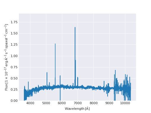
We can also slice a datacube to get a single spectrum
>>> spectrum_20_20 = flux[:, 20, 20]
>>> spectrum_20_20
<Spectrum [0.0669153, 0.0599907, 0.0229852, ..., 0.       , 0.       ,
       0.       ] 1e-17 erg / (Angstrom cm2 s spaxel)>
In this case the returned Quantity is a 1D Spectrum. This new Quantity behaves exactly as the DataCube but in this case we can also plot the spectrum
>>> spectrum_20_20.plot()
<matplotlib.axes._subplots.AxesSubplot at 0x130a1d518>
(Source code, png, hires.png, pdf)
Let’s now have a look at the Marvin 2D Quantity: the Map.
>>> maps_obj = Maps('7443-12703')
>>> ha = maps_obj.emline_gflux_ha_6564
<Marvin Map (property='emline_gflux_ha_6564')>
[[0. 0. 0. ... 0. 0. 0.]
[0. 0. 0. ... 0. 0. 0.]
[0. 0. 0. ... 0. 0. 0.]
...
[0. 0. 0. ... 0. 0. 0.]
[0. 0. 0. ... 0. 0. 0.]
[0. 0. 0. ... 0. 0. 0.]] 1e-17 erg / (cm2 s spaxel)
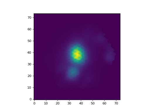
We can still use all the tools we discussed above. For example, let’s plot the signal-to-noise ratio
>>> snr = ha.snr
>>> plt.imshow(snr, origin='lower')
(Source code, png, hires.png, pdf)
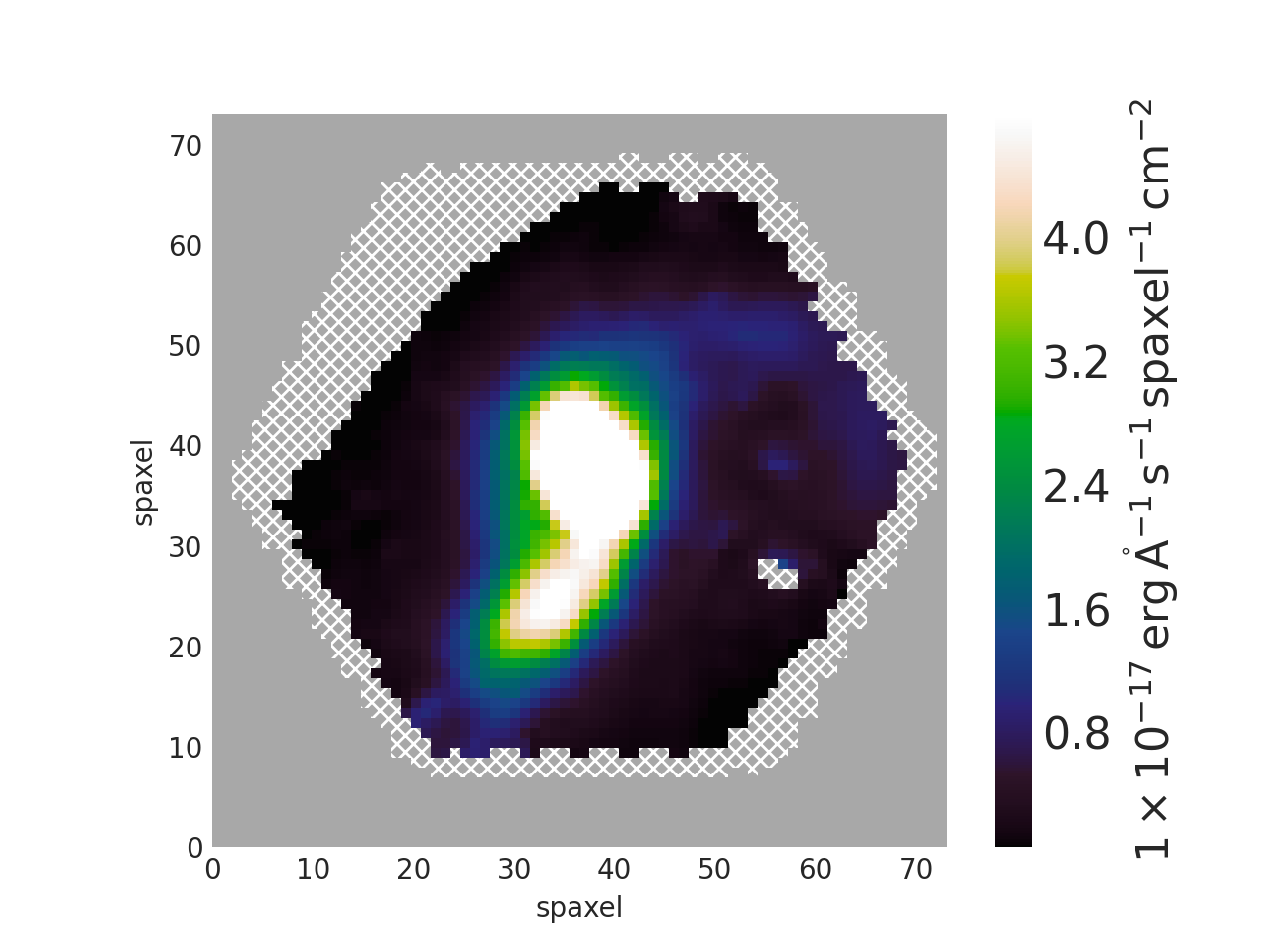
Map objects are a bit special, though, and we will discuss them in detail in their own section. Here, let’s see how we can do “Map arithmetic” by calculating the \({\rm H\alpha/H\beta}\) ratio
>>> hb = maps_obj.emline_gew_hb_4862
>>> ha_hb = ha / hb
>>> ha_hb
<Marvin EnhancedMap>
array([[nan, nan, nan, ..., nan, nan, nan],
       [nan, nan, nan, ..., nan, nan, nan],
       [nan, nan, nan, ..., nan, nan, nan],
       ...,
       [nan, nan, nan, ..., nan, nan, nan],
       [nan, nan, nan, ..., nan, nan, nan],
       [nan, nan, nan, ..., nan, nan, nan]], dtype=float32) '1e-17 erg / (Angstrom cm2 s spaxel)'
>>> ha_hb.plot()
(Source code, png, hires.png, pdf)

EnhancedMap result from the arithmetic combination of two maps and take care of all the gritty details: error propagation, division by zero, maskbit propagation, etc.
Finally, AnalysisProperty are 1D quantities associated with a value for a single spaxel on a Map. We will discuss them in depth when we talk about marvin-subregion-tools.